Visualizing slow turn-on time of long life energy saving bulbs
Background
When I bought my hallway lamp a few years ago, I fitted it with energy saving light bulbs. Little did I know that those specific bulbs turned on really slow. I’ve always felt that it took ages before the light output gets close to its final value, and finally I decided to actually measure it as well.
Presenting the result
There are a few different ways to present the results.
- One would be to simply play back the 20 minute video, but with a large speedup.
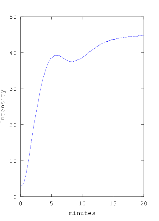
- Another would be to simply show the intensity vs time plot
- My approach was to combine both of them.
Combining both the video frame, and an animated plot:
Measurement setup
I used a Logitech C615 web camera. It has the ability to lock all settings to manual mode, so the camera won’t adapt to changes in the environment. That meant that I could set it up for a decent image after the hallway lamp had been running for an extended period of time, turn the lamp off for an hour, and then record a video where one would see how the hallway lamp slowly turns on.
Analyzing the video
I started by extracting one frame every second from the video file using ffmpeg
ffmpeg -i /media/slow_hall_lamp.mp4 -r 1 output_%06d.pngSince I’m working in octave quite often (a tool that aims to be matlab compatible), I decided to use octave for graphing. At first, I checked the same square in each and every image to get the intensity. The three lamps turned out to differ a bit in how fast they turned on, so I changed strategy.
The final strategy was to take the mean of almost all pixels in each video frame. The only pixels I excluded was those with an intensity exceeding the gray level value 200 in the final (brightest) frame, and pixels far to the right of the lamp.
Source code:
%
% Octave script used for generating a visualization of slow turn-on time
% of long life energy saving bulbs
%
% Copyright (c) 2014-2015 Simon Gustafsson (www.optisimon.com)
%
%
% Notes about the work flow needed to generate the video:
%
% 1) Extract an image every second from a video stream:
%    ffmpeg -i /media/slow_hall_lamp.mp4 -r 1 output_%06d.png
%
% 2) Run this script. Make sure in_folder, out_folder, and plot_folder
%    points to existing folders, and that the in_folder isn't empty.
%
% 3) ffmpeg didn't want to read the images unless they was numbered from zero
%    (but this scripts first image was 17, so i'm just reusing that image)
%    for var in `seq 0 16` ; do cp combined_000017.png combined_`printf %06g $var`.png ; done
%
% 4) converting the movie into something that windows media player / vlc / virtualdub can use
%    avconv -r 24 -f image2 -i /home/simon/combined/combined_%06d.png -vcodec rawvideo -r 24 -pix_fmt bgr24 output.avi
%
% 5) Could not use the video in the video editor directly (Movie Studio Platinum 12.0),
%    so had to run it once through VirtualDub (still raw output, but fast reprocessing...)
%

page_screen_output(0);

in_folder = "slow_hall_lamp"
out_folder = "combined"
plot_folder = "plot"

% Needed to revert to using gnuplot for graphs on my ubuntu 14.04
% installation. (seems like newer versions of octave are using an opengl
% backend for plotting graphs, which refused to print the plots with my
% requested dimensions)
graphics_toolkit("gnuplot")

function plot_fname = plot_and_save(n, vals, plot_folder)
  plot([0:length(vals)-1]./60, vals)

  % Axis limits are magic values, found by plotting all the
  % vals when every frame had been processed.
  axis([0 20 0 50 0 1])

  xlabel("minutes");
  ylabel("Intensity");

  minutes = floor(n / 60);
  seconds = n - 60*minutes;
  title(sprintf("%02d:%02d [mm:ss]", minutes, seconds))

  plot_fname = sprintf("%s/graph_%06d.png", plot_folder, n);

  % Save the plot on the file system.
  %
  % Height 720 works in ubuntu 14.04 with octave 3.8.1 and gnuplot 4.6.4,
  % but I had to use heght 721 when running stock versions of tools in
  % ubuntu 12.04, so keeping a height of 721 here as a workaround for others.
  print(plot_fname, "-S522,721");
end


% Calculate a mask, so regions close to saturation won't influence
% measured intensities
X=imread("slow_hall_lamp/output_001214.png");
X2=mean(X,3);
include_mask = (X2 <= 200);
include_mask(:,743:end) = 0; % Also mask away right side of image

figure(1);
imshow(include_mask);
title("include mask");


figure(2);
files=glob([ in_folder "/output_*.png"]);
vals = [];

for n=17:length(files) % from 17 to disregard the very first frames
  filename=files{n}

  % Read webcam image
  X=imread(filename);

  % Convert to gray scale, not accounting for perceived brightness
  X2=mean(X,3);

  % Get mean intensity of current frame (excluding masked regions)
  masked_img = include_mask .* X2;
  v = mean(masked_img(:))

  % Keep track of all intensities so far
  vals = [vals; v];

  % Graph all current intensity values, and save the plot as an image.
  % Magic number -17 since I wanted to skip the first 17 frames
  % (and we don't want seconds to start at 17)
  plot_fname = plot_and_save(n-17, vals, plot_folder);

  % Read back the plotted graph
  X_plot = imread(plot_fname);
  if size(X_plot,3) == 1
    % Oh, image library tries to be smart, won't waste bits for color if
    % a color image happens to only have black and white pixels
    X_plot(:,:,1) = X_plot;
    X_plot(:,:,2) = X_plot(:,:,1);
    X_plot(:,:,3) = X_plot(:,:,1);
  end

  % Combine the webcam image and the graph of current intensity values
  X_combined = X;
  % Doing strange thing since plotted image didn't want to be
  % 720 pixels in height...
  X_combined(:,end-size(X_plot, 2)+1:end,:) = X_plot(1:720,:,:);

  % Save the combined image containing the webcam image and the plot.
  combined_fname = sprintf("%s/combined_%06d.png", out_folder, n);
  imwrite(X_combined, combined_fname);
end
Graph
For reference, the last intensity vs time graph is included here as well